

If it were not enough that investors are digesting less than stellar second quarter earnings, they are also dealing with the mixed seasonal patterns unique to August. August tends to be a mediocre month for stocks, with no strong directional bias. Some indices might see slight gains, while others could experience declines. This lack of a clear trend makes August a bit of a coin flip for investors.
It’s like picking a suitcase on Deal or No Deal… never knowing what you will get. Not knowing can be half the fun or more likely half the frustration. This August is following the same seasonal pattern, despite some over-the-top intraday volatility.
To that point, we recognize that underpinning stock selection is the inability to predict emotional short-term responses to macro events. Affectionately referred to as the “Fire, Aim, Ready” axiom. Case in point, August 5th, when the Dow Jones Industrial Average fell more than 1,000 points within the first hour of trading.
Keeping with the fire, aim, ready truism, investors typically sold first without really knowing why. While there were three explanations for the sell-off, the one fact that stood out to us was the SPX (S&P 500) closing price of 5,163.10 (the low point when stocks opened for trading on August 5th of the day. See chart.). That closing value was approximately 10% below the most recent high, which is what we would expect to see in a normal correction. The market bounced off that level on Tuesday and held above the low point for the remainder of the week.
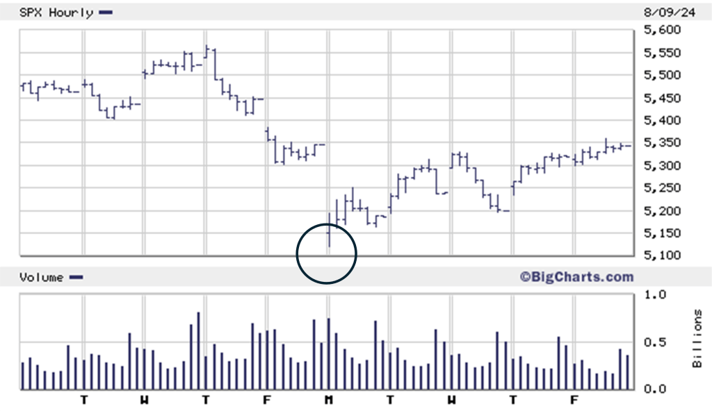
The challenge for investors is not related to the typical correction. It is more about the speed at which the correction took place. Experiencing a 10% correction in three to five days rather than over a period of one to two months takes a considerable emotional toll.
Because of that, we believe it is important to put some meat on this skeleton by shedding light on the three factors that caused the sell-off. They include the trigger, which was the carry trade, the explanatory positioning which was the unemployment report (notably the Sahm Rule), and the rotation shift which was the macro momentum factor.
THE CARRY TRADE
Imagine borrowing free money and using that capital to buy securities that provide a positive yield. Seems too good to be true, but it was this unusual set of events that supported the Yen carry trade.
Large institutional hedge funds began investing in this strategy in 2022, when inflation became a problem for most industrialized economies. Japan, with its unique demographic, being the exception.
As inflation spiked – except in Japan – central banks began raising interest rates to quell excess demand as household’s were flush with cash from pandemic induced government stimulus.
The Bank of Japan was the outlier holding interest rates at or near zero to combat stubborn deflationary influences that had gripped the economy. In fact, during the early stages of the carry trade Japan, was experiencing negative interest rates.
Hedge funds pounced on this aberration by borrowing Yen (i.e. to borrow Yen, funds would sell Japanese bonds) and using that free capital to buy positive yielding assets like US treasuries and for the managers looking for more aggressive exposure, buying the magnificent seven stocks.
Not surprisingly, since hedge funds are paid for performance, leverage was employed to pump up returns. The carry trade became so popular that at one point, analysts estimated that more than a Trillion dollars was committed to the strategy.
That may seem like a big number, and it is, but foreign exchange and fixed income markets represent the majority of available capital in the global sphere. The size and scale of these markets dwarf the global equity space.
The main risks in a carry trade are changes in the exchange rate and interest rate differential. If, rates rise in Japan and the Yen appreciates against foreign currencies, it can eliminate the profit from the interest rate differential. Depending on the size of the move, it can reduce the gains or even turn them into losses.
A tsunami swept over the carry trade on July 31st when the Bank of Japan decided to raise interest rates from 0.10% to 0.25%. The Yen surged against the US dollar and Japanese bonds attracted a bid.
This caused an epic unwinding of the yen-funded carry trade that wreaked havoc across global markets. The strategy which kept money flowing into global risk assets for years forced investors to abandon the trade as the yen surged higher. The Japanese equity markets had their worst day since 1987.
At the same time, US bonds resetting based on expectations for a September rate cut and US equity investors were mired in a rotation out of the magnificent seven tech stocks into more value-oriented plays like consumer staples, healthcare, small cap stocks and financials. This sea change triggered a rush to the exits which we suspect caused the capitulation when stocks opened for trading on August 5th.
There may be more to come because the carry trade operates in an institutional space. Prices are set by reams of institutional traders who can buy sizeable blocks to assist with the unwinding process. The best guess is that 50% to 60% of the carry trade has been unwound. We suspect, at this stage, that most of the inherent leverage has been removed. If that assumption is correct, any further downside should be manageable.
THE SAHM RULE
The “Sahm Rule,” named after macroeconomist Claudia Sahm[1], is an economic indicator that attempts to highlight the preliminary stages of a recession. Ms. Sahm introduced the indicator as part of a policy proposal called “Direct Stimulus Payments to Individuals.” The proposal, published by The Hamilton Project[2], was to inject government stimulus into the economy at the onset of a recession. If the stimulus was injected at the right time, it could shorten the recession’s timeline and reduce the economic impact.
It was an interesting line of attack if you favor a liberal course of action. Unfortunately, or fortunately (depending on your political bent), liberal policies are a tough sell in the US. As such, government stimulus never gained much traction.
Still, the concept was grounded in logic. When analyzing the ex-post trajectory of recessions, economists noted that most began with a marked slowdown in consumer spending. Likely as in the current environment, because inflation wreaked havoc on consumer’s disposable income. Not to mention angst – real or imagined – about a slowing jobs market.
Sahm believed that automatically injecting government stimulus payments to families at the onset of a recession would dramatically reduce the impact of higher unemployment that invariably accompanies a downturn. The challenge was trying to time the stimulus injection. Predicting the onset of a recession is like trying to predict the weather. There are simply too many variables that are subject to sudden changes.
The Sahm Rule was designed as a tool to predict the onset of a recession which she defined as a point at which the three-month average national employment rate jumps at least half a percentage point relative to its low over the last 12 months.
What makes the Sahm Rule interesting is its’ simplicity and ability to quickly reflect the onset of a recession. According to the Sahm Rule, the early stage of a recession is signaled when the three-month moving average of the U.S. unemployment rate is half a percentage point or more above the lowest three-month moving average unemployment rate over the previous twelve months.
The unemployment rate represents the percentage of the overall labor force that is unemployed. The rate tends to rise when the economy is struggling, and workers are having difficulty finding jobs and falls when the economy is strong and workers can more easily find employment. The Bureau of Labor Statistics (BLS) typically releases the unemployment rate for the previous month on the first Friday of every month.
The Sahm rule compares the value of the current three-month moving average unemployment rate to the value of the lowest three-month moving average unemployment rate over the last twelve months. If the former is half a percentage point or more above the latter, the Sahm Rule indicates that the U.S. is in the initial stages of a recession. The Sahm Rule uses the three-month moving average unemployment rate – rather than the current unemployment rate – to prevent overreacting to a single month of data.
Since the early 1970s, the indicator has never been triggered outside of a recession, according to Sahm. Historically, when the unemployment rate passes the threshold outlined by the Sahm rule, it continues to increase. And we now come full circle. The Sahm rule was triggered, and investors reacted when the unemployment rate bumped higher on July 27th (see chart). The rule has historically proven to be very accurate. Since the 1970s, the Sahm Rule has always triggered in the early stages of a recession.
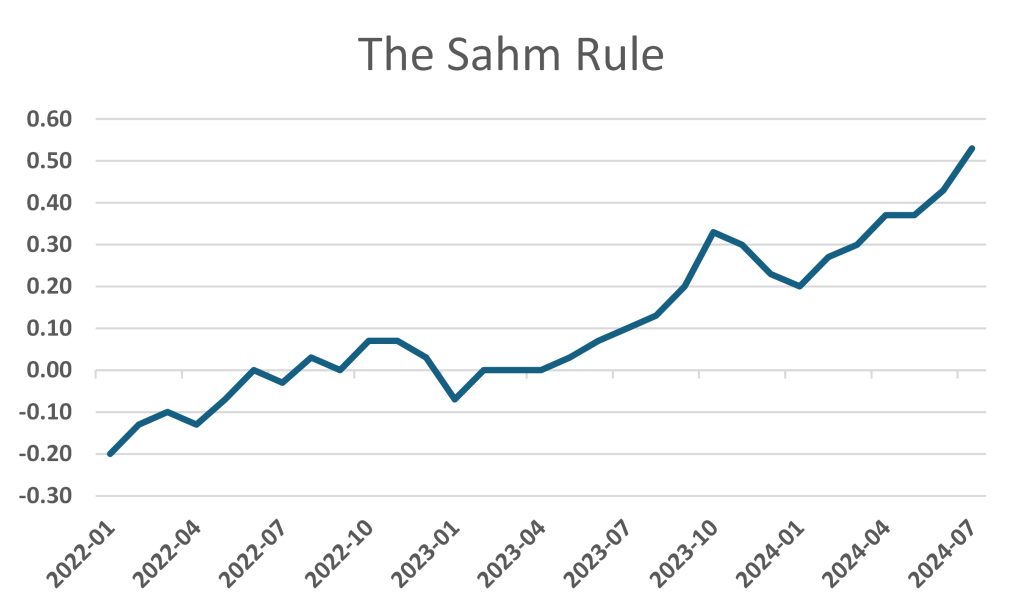
Investors were concerned, because if we are at the beginning of a recession, it could put the soft-landing scenario in jeopardy. That may be true, but be mindful that the Sahm Rule has limitations. Most notably, as Sahm pointed out in her newsletter, the rule is “empirical regularity,” not a proposition. She emphasized that this means that the rule can issue a false narrative.
For example, Sahm wrote in an April 2022 newsletter, imagine a scenario in which the unemployment rate increased to say 3.5%, up from a low of 3.0%, meeting the criteria for signaling the early stages of a recession. However, if around that same time, GDP growth held around 2.5%, down from a high of 5.5%, and inflation gradually slid down to 2%, such a combination of circumstances probably would not constitute a recession, she explained.
The recent slowdown in the U.S. job market touched off days of global stock-market turmoil also fueled speculation the Federal Reserve may not wait until its next scheduled meeting, in September, to cut interest rates.
Indeed, an interest rate futures contract expiring later this month that tracks Fed policy expectations recently shot to a two-month high implying that rates would be lower by the end of August.
MARKET ROTATION
Before the equity markets were spooked by the Sahm Rule and pummeled by the unwinding of the carry trade, traders were engaged in a rotation away from momentum stocks into more value plays and small cap companies.
The backdrop for this rotation was the notion that the Federal Reserve would begin cutting interest rates sooner than later. Lower rates would make it more cost-effective for smaller companies which would improve their profit margins.
Small cap stocks had been underperforming their large cap cousins since the end of the pandemic. Not surprising since larger companies had sizeable balance sheets and were earning decent interest on their cash hoard. Moreover, adding leverage would only have a minimal impact on their earnings per share, so there was no urgency to borrow. Small cap stocks, on the other hand, needed capital to grow which meant that higher rates hindered their bottom line.
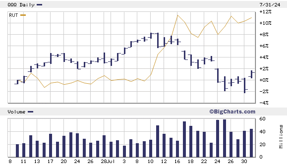
The market rotation was most pronounced among the mega-cap technology stocks. Analysts viewed this as a positive development because the market had become so concentrated. Unfortunately, these transitions can lead to enhanced volatility.
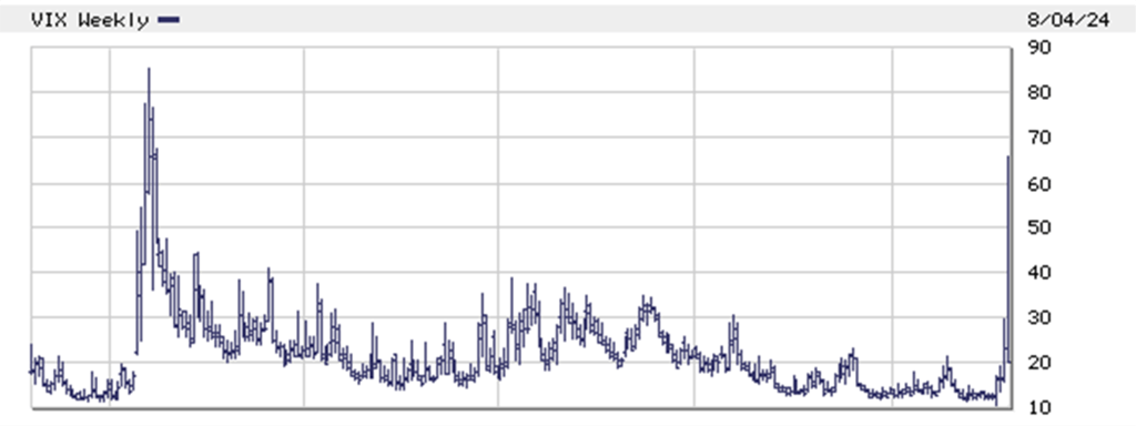
Volatility spiked as the early shift away from momentum stocks combined with the triggering of the Sahm rule and the unwind of the carry trade. At one point, the CBOE Volatility Index crossed 60, which had not been seen since the onset of the pandemic.
IMPLICATIONS FOR INVESTORS
In short, we are convinced that the Fed has a bias toward easing policy. Not surprisingly, given this view, Fed officials believe inflation is the result of various supply shortfalls in the economy, rather than demand fueled by factors like aggressive fiscal spending and excessive growth in the money supply.
According to Morgan Stanley, “this bias is now being tested and odds are rising that the Fed’s apparent objectives around financial liquidity and market stability will be exposed.” In this environment, portfolio diversification is key.
The advantage when confronted with a combination of cross-currents is that it provides an opportunity to re-balance portfolios, taking profits in richly valued equities while adding some exposure to high-quality fixed income without much need to invest in longer-duration assets to find attractive yield
TRADITIONAL VS ENHANCED INCOME MANDATES
A central theme in portfolio management is risk-adjusted return. Weighing potential upside performance against downside variability.
Most investors understand the performance side of the equation. Simple arithmetic: set an objective, determine the time horizon, and calculate the required rate of return.
Risk is more subjective. We can measure risk by calculating a portfolio’s variability over a specific period. But knowing a portfolio could experience x% downside variability sheds no light on how investors are likely to react.
Notionally, we can use questionnaires to determine an investor’s risk tolerance. The reality: measuring risk tolerance ex-ante is like trying to guess Wayne Gretzky’s next move based on his latest trajectory. It might be better than a blind guess, but not by much.
The risk question is especially relevant for income portfolios. Having its own nomenclature with risk being defined as the “age of ruin,” it comes down to how long the portfolio can fund the investor’s needs and wants before it runs out of money.
Income mandates are conservative as they appeal to retired seniors who, by definition, have a low tolerance for risk. Conservative income portfolios are typically over-weighted in fixed income securities (i.e. bonds and preferred shares) with a limited allocation to equities.
But does an overweight bond allocation reduce risk? Bond prices move inversely to interest rates. Rising rates lower bond prices, declining rates, higher bond prices! When interest rates were at or near zero during the Covid pandemic, it was hard to imagine any scenario where bonds would reduce risk within a portfolio. In fact fixed income assets – i.e. bonds and preferred shares – could be categorized as the highest risk asset class within a portfolio. Risk exacerbated on a sliding scale that corresponded to the term to maturity.
Much has changed with the unprecedented spike in rates as global central banks attempted to slow an inflationary spiral. In the current market, where rates are expected to decline over the next eighteen months, bonds and preferred shares now represent the ballast that reduces risk within income mandates.
The challenge for income seeking investors is to balance the underperformance of traditional income mandates against the surge in growth assets that typically reside in the momentum camp. Developing sustainable income portfolios in the current growth environment means altering one’s perception of risk. Looking past stock price performance price while focusing instead on income sustainability.
Easier said than done! Extended periods of underperformance, which has been the hallmark of income mandates, can be catastrophic, often leading to bad decisions based on emotions… notably fear and greed. However, an income portfolio that may produce upside share price performance, with minimum price variability that is unable to generate stable cashflow will lead to principal drawdowns that in the long term, will negatively impact the age of ruin timeline.
We can manage bad behavior caused by short term price swings, by recognizing that variability varies by time (i.e. the length of time you hold an investment). Looking at long term performance data makes short term aberrations seem inconsequential. The key is being comforted by the knowledge that solid blue-chip value stocks will recover in time. More importantly, this group of stocks typically increase dividends, which not only supports their stock price but also provide the required income that meets most if not all, of the initial income objective.
THE IMPACT OF PRINCIPAL DRAWDOWNS
We have found that generally, the income needs for most retirees exceeds the cashflow being generated by the allocation within a traditional income portfolio (i.e. 50% stocks, 50% fixed income). To offset the shortfall, the portfolio manager must sell assets which necessitates a drawdown of principal. For many retirees, the drawdowns outweigh the advantages of reduced variability and higher share prices.
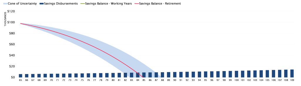
Think about it this way. Suppose you have $100,000 in laddered GICs yielding 4% per annum. That portfolio will generate $4,000 per year in income with no tax benefit. If at age 65, your required annual income is $6,000 adjusted annually for a 1% inflation rate, you will be drawing down principal at a rate of $2,000 per year. The portfolio will have zero variability, with a guarantee that you will run out of money before age 85 (see figure 1).
Figure 1: Portfolio Depletion: Laddered GIC Portfolio
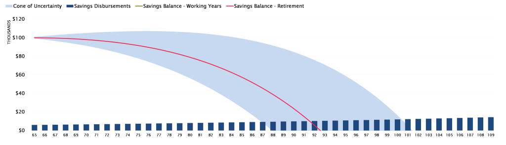
If the retirees’ principal is being disproportionately eroded, a portfolio generating more income with heightened price variability, may be the better approach. Using the same analogy, suppose a hypothetical $100,000 portfolio that includes dividend paying stocks and option writing strategies produces $5,000 per year in tax-advantaged cash flow.
Managing the shortfall requires an annual drawdown of $1,000. This drawdown is less intrusive, but it can be painful if it occurs at a time when the portfolio is experiencing a sharp sell-off.
To shed light on potential pitfalls linked to Enhanced Income portfolios, we incorporate a “cone of uncertainty” bracketing best and worst-case scenarios. In this example, because drawdowns are less intrusive, the Enhanced Income portfolio should be sustainable until at least age 92 and could last a lifetime.
Figure 2: Portfolio Depletion for the Enhanced Income Portfolio
There lies the trade-off! Is a minimum volatility portfolio appropriate if you are forced to draw down excess principal? Or does a higher yielding, potentially more volatile model where the underlying components are more tax-efficient (capital gains and dividends versus interest income) and offer the potential of higher payouts over time (i.e. dividend increases) provide a better solution for income-oriented investors?
AFTER TAX RETURN
How do taxes fit into this discussion? Interest income is taxed as ordinary income which means you pay the marginal tax rate on total cash flow. Dividends from common and preferred shares and capital gains from option writing strategies are more tax efficient which may require less of a drawdown to end up with the same after-tax cash flow.
Going back to our previous example, $6,000 of interest income on the hypothetical $100,000 GIC portfolio will, depending on your marginal tax rate, deliver approximately $4,000 of after-tax income. The alternative income model delivering the same $6,000 in dividend and capital gain income will leave you with about $4,800 in after tax income.
And what about inflation? A reluctance to deal with significant government deficits have historically, been inflationary. Cost of living adjustments to your monthly income can have an outsized impact on principal drawdowns. Rising dividend payouts act as a counter-weight to those risks.
In our experience most investors cannot survive on the income generated by a laddered GIC portfolio or an annuity. It simply does not generate enough cashflow and cannot effectively offset inflation expectations. In the real world, we need to step outside the GIC and annuity spectrum, into either a more traditional income allocation (50% stocks, 50% fixed income) or a more tax-efficient alternative Income model that focuses on value stocks with solid dividends, preferred shares, and bonds bolstered by option writing strategies.
Choosing a traditional versus alternative Income approach rests with investors’ ability to tolerate increased portfolio variability. The alternative Income model theoretically carries greater risk both in terms of price variability and the fact that corporations can withhold dividends to shore up balance sheets (note: management determines whether to pay or withhold a dividend which hinges on current economic trends).
We can deal with the second element by selecting companies where there is a high degree of probability that the dividends will be maintained. Ideally, we want companies that have increased dividends over time thus providing the best of both worlds. Investors enjoy the tax advantages that come with dividends and benefit from increased cash flow that supports inflation adjustments.
The variability question hinges on the investors’ risk tolerance which is more theoretical than factual. For one thing, the reduced variability in the traditional income model assumes that bonds and GICs are a low-risk alternative which is not always the case. Still, an equity-based portfolio that pays dividends supplemented by a well thought out option writing program will, by definition, be more volatile.
Unfortunately, for portfolio managers we rarely know how much variability a client can absorb until the investor experiences downside price action or extended periods of underperformance. The Advisor’s job is to help manage the emotional roller-coaster so the investor can weigh the benefits versus the risk and hopefully, stay the course until better times emerge.
SUMMARY
The alternative income model is a viable option for certain investors. It will appeal to investors where their required income can be attained without significant drawdowns on principal.
It is appropriate for investors who think about the alternative income model in much the same way as they think about a pension plan. To that point, investors must have a pre-defined and consistent income objective. One would not make one-off requests for funds from their pension administrator. That same discipline must apply to the alternative income mandate.
Periodic requests for supplemental withdrawals typically result in asset sales (i.e. principal drawdowns). Usually, these sales occur during market declines which historically have had a profound impact on the viability of the strategy.
Ideally income investors who are willing to gravitate to this type of model would define their required income needs within the context of the cash flow being generated by the model. On that note, one should set their required income at a rate that is not greater than 70% of the cashflow being generated by the portfolio. For example, if the portfolio generates $5,000 annually through dividends and distributions, the required annual income should not be greater than $6,500.
Investor behavior is also critical. Those who can focus on the stability of the cash flow while discounting the variability of monthly and yearly return data will be in a better position to reap the many benefits of the alternative model. To that point, I encourage investors to immediately begin drawing monthly income. Ideally, the consistency of the cash flow will in time (usually six to eighteen months) alleviate concerns about portfolio variability.
That latter point is particularly relevant during the initial “black swan” sell-off during the pandemic shutdown. While the decline was draconian, it had no impact on the portfolios’ cash flow. Proving once again, that the worst thing one can do is exit a viable long-term strategy because of a short-term aberration.

Richard N Croft
Chief Investment Officer
[1] Claudia Sahm worked at the US Federal Reserve and served on the White House Council of Economic Advisors.
[2] The Hamilton Project is a think tank at the Brookings Institution.